// method
Aperture bias corrections
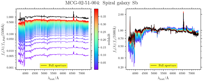
SDSS spectra are collected through a fixed 3″ fiber, which captures only the
central region of nearby galaxies. Because stellar population gradients are
common — galaxies tend to have older, more metal-rich centres — the fiber
systematically misrepresents the integrated light, biasing the inferred
stellar population parameters. BaStA corrects for this
fiber-aperture bias before fitting, using a procedure
calibrated on spatially resolved CALIFA integral-field observations
(Zibetti et al. 2026).
core strategy
For each spectral index, the correction from fiber to integrated value is
modelled as a smooth function of four observable parameters: the
index measured in the fiber, the global
g−r colour, the
r-band
effective radius Re, and the
absolute r-band magnitude. These four quantities
together capture the diversity of aperture corrections with high accuracy,
without requiring detailed morphological classification.
Two-step correction procedure
The procedure is applied independently at each redshift on a grid spanning
0.005 < z < 0.4, using CALIFA galaxies as the
calibration sample. For each galaxy and each index, the difference
ΔX between the integrated and fiber values is modelled in
two successive steps:
1st order
Index in fiber & global colour
The systematic variation of ΔX across the plane of
fiber-index versus total g−r colour is regularised
using a 2D LOESS regression. This first-order
correction removes most of the systematic bias — in the case of
HδA+HγA, a median
offset of ~1.4 Å is reduced to negligible levels.
2nd order
Effective radius & absolute magnitude
Residual trends in the first-order corrected values are visible in the
plane of Re versus absolute magnitude. A second
LOESS regression in this plane provides a refinement correction that
substantially reduces the tail and skewness of the
residual distribution, even when the median bias is already small.
Applying corrections to SDSS galaxies
The correction functions are defined on the discrete set of CALIFA
galaxies. Local smoothing and 3σ rejection loops regularize these functions and remove
outlier CALIFA galaxies. To extend them to any point in the planes of
fiber-index versus total g−r colour and of Re versus absolute magnitude
(for any SDSS galaxy), a
nearest-neighbour interpolation is used, with distances
defined by an observationally motivated metric that weights each parameter
by its measurement uncertainty:
distance metrics
1st-order plane — fiber index & g−r colour:
d1,i = √[ (Δg−r)2 / σ2g−r +
(ΔX)2 / σ2X ]
2nd-order plane — size & luminosity:
d2,i = √[ (ΔMr)2 / σ2Mr +
log2(R50,obs / R50,i) / σ2log R50 ]
The two correction terms are found independently — the nearest neighbour
in the first-order plane need not be the same galaxy as in the second-order
plane. This allows each correction to use the most relevant information
available for each object.
At each step, a 3σ rejection algorithm removes
outlier CALIFA galaxies from the calibration before the corrections are
finalised. Typically only a handful of galaxies per index per redshift are
excluded. Crucially, the scatter in the residuals after correction is
smaller than the typical SDSS measurement uncertainties,
meaning that aperture correction errors contribute negligibly to the
final error budget.